6.1.1 Possibility of video signal compression
This article refers to the address: http://
There is a large amount of redundancy in the video data, that is, there is a strong correlation between the pixel data of the image. Using these correlations, the data of a part of the pixels can be derived from the data of another part of the pixels, and as a result, the amount of video data can be greatly compressed, which is advantageous for transmission and storage. Video data mainly has the following forms of redundancy.
1. Spatial Redundancy Video images vary generally between adjacent pixels in the horizontal direction and between adjacent pixels in the vertical direction, and there is a strong spatial correlation. In particular, there is often spatial coherence between grayscale and color at each point of the same scene, resulting in spatial redundancy, often referred to as intraframe correlation.
2. Time Redundancy There is a strong correlation between luminance and chrominance information between adjacent pixels in adjacent fields or adjacent frames. The current frame image tends to have the same background and moving objects as the first and last frames, but the spatial position of the moving object is slightly different. For most pixels, the brightness and chrominance information are basically the same, called Inter-frame correlation or time correlation.
3. Structural Redundancy In some texture regions of the image, the pixel values ​​of the image have a distinct distribution pattern. Such as a checkered floor pattern. Knowing the distribution pattern, an image can be generated by a process called structural redundancy.
4. Knowledge Redundancy Some images have a considerable correlation with certain knowledge. For example, the image of the face has a fixed structure, the nose is above the mouth, the eyes are above the nose, and the nose is located on the midline of the facial image. Such regular structures can be obtained from prior knowledge, and such redundancy is called knowledge redundancy.
5. Visual redundancy The human eye has visual non-uniform characteristics, and information that is not sensitive to vision can be appropriately discarded. When recording raw image data, it is generally assumed that the visual system is linear and uniform, treating visually sensitive and insensitive parts equally, resulting in coding that is more distinct than ideal coding (ie, distinguishing between visually sensitive and insensitive parts). ) More data, this is visual redundancy. The human eye does not have the highest resolution for image detail, amplitude variation, and image motion.
Human eye vision is interchangeable for the spatial resolution of the image and the time resolution force. When one party is required to be higher, the requirement for the other party is lower. According to this feature, motion detection adaptive technology can be used to reduce the time-axis sampling frequency of still images or slow moving images, for example, one frame every two frames; and reduce the spatial sampling frequency for fast moving images.
In addition, the requirements of the human eye vision for the spatial and temporal resolution of the image and the requirements for the amplitude resolution force are also interchangeable. There is an appreciable threshold for the amplitude error of the image, which is lower than the threshold error. Undetected, near the edge (contour) or time edge of the image (the moment of sudden change of the scene), the perceived threshold is 3 to 4 times larger than the distance from the edge. This is the visual masking effect.
According to this feature, the edge detection adaptive technique can be used to fine-tune the coefficients of the low-frequency components of the image after the gradual region or orthogonal transformation of the image, and coarsely quantize the coefficients of the high-frequency components of the image after the image contour or orthogonal transformation; The coarse quantization is performed when the interframe predictive coding rate is higher than the normal value due to the fast motion of the scene, and vice versa. In the quantification, try to make the amplitude error generated in each case just below the perceptible threshold, which can achieve higher data compression rate and subjective evaluation.
6. Identity redundancy of image regions All pixel values ​​corresponding to two or more regions in the image are the same or similar, resulting in data repetitive storage, which is the similarity redundancy of image regions. In this case, the color values ​​of the pixels in one region are recorded, and the regions of the same or similar are no longer recorded for each pixel. The vector quantization method is a compression method for such redundant images.
7. Statistical redundancy of textures Although some image textures do not strictly obey a certain distribution law, they obey the law in a statistical sense. By using this property, the amount of data representing the image can also be reduced, which is called statistical redundancy of texture.
The information redundancy existing in the television image signal data provides a possibility for video compression coding.
6.1.2 Digitization and compression of video signals The process of encoding, quantizing and encoding a television signal (including video and audio) into a binary digital signal is called analog-to-digital conversion (A/D conversion) or pulse-coded modulation (PCM, Pulse Coding). Modulation), the resulting signal is also referred to as a PCM signal, and the process can be represented by Figure 6-1(a). If the sampling frequency is equal to fs and quantized with n bits, the code rate of the PCM signal is nfs (bits/s). The PCM code can be performed either directly on the color full television signal or separately on the luminance signal and the two color difference signals. The former is called full signal coding, and the latter is called component coding.
The PCM signal is decoded and converted into an analog signal by decoding and insertion filtering. As shown in Figure 6-1(b), decoding is the inverse of encoding. Insertion filtering is to interpolate the decoded signal into a smooth, continuous analog signal. These two steps are collectively referred to as digital to analog conversion (D/A conversion) or PCM decoding.
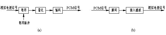
Figure 6-1 Digitization and restoration of TV signals (a) A/D conversion; (b) D/A conversion
1. Nyquist sampling theorem Ideal sampling, as long as the sampling frequency is greater than or equal to twice the highest frequency in the analog signal, the analog signal can be recovered without distortion, called the Nyquist sampling theorem. The double of the highest frequency in the analog signal is called the folding frequency.
2. The Nyquist sampling is based on the sampling theorem. If the sampling frequency fs is less than 2 times the maximum frequency fmax of the analog signal, aliasing distortion will occur. However, if the sampling frequency is skillfully selected, the aliasing component in the sampled spectrum will fall. Between the chrominance component and the luminance component, the aliasing component can be removed by a comb filter.
3. Uniform Quantization and Non-Uniform Quantization Quantization in which the quantization interval amplitudes are equal within the dynamic range of the input signal is called uniform quantization or linear quantization. For uniform quantization with fixed quantization spacing, the signal-to-noise ratio increases with the increase of the input signal amplitude. When the signal is strong, the noise can be submerged. In the case of weak signals, the interference of the noise is very significant.
In order to improve the signal-to-noise ratio of weak signals, the quantization pitch should vary with the amplitude of the input signal, coarse quantization is performed for large signals, and fine quantization is performed for small signals, that is, non-uniform quantization (or nonlinear quantization) is employed.
There are two methods for non-uniform quantization. One is to place the nonlinear processing in the analog part before the encoder and after the decoder. The encoding and decoding still use uniform quantization. Before the uniform quantization of the encoder, the input signal is compressed. It is effective for coarse quantization of large signals, and small signals for fine quantization; after uniformly quantizing the decoder, it is expanded to restore the original signal. Another method is to directly use a non-uniform quantizer, which performs coarse quantization when the input signal is large (large quantization spacing), and the input signal is finely quantized (quantization pitch is small). There are also a number of uniform quantizers with different quantization pitches. When the input signal exceeds a certain level, it enters the coarse pitch uniform quantizer. When it is below a certain level, it enters the fine pitch quantizer, which is called quasi-instantaneous companding.
Usually, Q is used for quantization, and Q-1 is used for inverse quantization. The quantization process is equivalent to finding the interval number in which it is located from the input value, and the inverse quantization process is equivalent to obtaining the corresponding quantization level value from the quantized interval number. The total number of quantization intervals is much less than the total number of input values, so quantization can achieve data compression. Obviously, the inverse quantization does not guarantee the original value, so the quantization process is an irreversible process. The quantization method is a non-information-preserving code. Usually these two processes can be implemented by the look-up table method, the quantization process is completed at the encoding end, and the inverse quantization process is completed at the decoding end.
The encoding of the quantized interval label (quantized value) generally adopts an equal length encoding method. When the total number of quantization layers is K, the quantized compressed binary digital rate is lbK bits/magnitude. In some high-demand situations, variable word length coding such as Huffman coding or arithmetic coding can be employed to further improve coding efficiency.
6.1.3 ITU-R BT.601 component digital system Digital video signals are formed by sampling, quantizing and encoding analog video signals. Analog TVs have PAL, NTSC, etc., which will inevitably form digital video signals of different standards, which is not convenient for intercommunication of international digital video signals. In October 1982, the International Radio Consultative Committee (CCIR) adopted the first proposal for digital encoding of studio color television signals. In 1993, it was changed to ITU-R (ITU Radiocommunication Sector, International). Telecommunications Union-Radio communications Sector) BT.601 component digital system recommendations.
BT.601 proposes a component coding method for separately encoding the luminance signal and the two color difference signals. The same sampling frequency is 13.5 MHz for signals of different standards, and the luminance signal Y is sampled regardless of the color subcarrier frequency of any standard. The frequency is 13.5 MHz. Since the bandwidth of the chrominance signal is much narrower than the bandwidth of the luminance signal, the sampling frequency for the chrominance signals U and V is 6.75 MHz. Each digital active line has 720 luma samples and 360 x 2 color difference signal samples, respectively. The sampling points for each component are uniformly quantized, and 8-bit precision PCM encoding is performed for each sample.
These parameters are the same for 525 lines, 60 fields/second, and 625 lines of 50 fields/second. The effective sampling point means that only the sample of the line and field scanning forward is valid, and the sample of the reverse is not within the range of the PCM encoding. Because in the digitized video signal, the line, field sync signal and blanking signal are no longer needed, as long as there is a starting position of the line and field (frame). For example, for PAL, it takes about 200 Mb/s to transfer all sample data, and only 160 Mb/s is needed to transfer valid samples.
The sampling rate of the chrominance signal is half of the sampling rate of the luminance signal, which is often referred to as the 4:2:2 format. It can be understood that the ratio of the number of samples of Y, U, and V in each line is 4:2:2.
6.1.4 Entropy Coding Entropy Coding is a type of lossless coding, named after the coded average code length is close to the entropy of the source. Entropy coding is implemented by variable length coding (VLC). The basic principle is to assign a short code to a symbol with a high probability of occurrence in a source, and a long code to a symbol with a small probability of occurrence, thereby obtaining a statistically shorter average code length. The code to be coded should be instant decodable, and one code will not be the prefix of another code, and the codes can be separated naturally without additional information.
1. Huffman coding Huffman coding is a variable length coding, as shown in Figure 6-2.
(1) Arrange the input signal symbols in a column with the probability of occurrence from large to small.
(2) Combine the two minimum probability symbols into a new probability, and then sort by the size of the probability of occurrence.
(3) Repeat step (2) until there are only two probabilities left.
(4) The coding proceeds from the last step step by step. The symbol with high probability is given the “0†code, and the other probability is given the “1†code until the initial probability arrangement is reached. 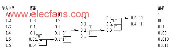
Figure 6-2 Huffman coding
2. Arithmetic coded Huffman code uses an integer bit for each code. If a symbol only needs to be represented by 2.5 bits, it must be represented by 3 symbols in Huffman coding, so its Less efficient. In contrast, arithmetic coding does not produce a separate code for each symbol, but instead causes the entire message to share a single code, and each new symbol added to the information incrementally modifies the output code.
Assume that the source consists of four symbols S1, S2, S3, and S4. The probability model is shown in Table 6-1. The probability of occurrence of each symbol is expressed in the unit probability interval as shown in Figure 6-3. The width of the interval represents the magnitude of the probability value, and the boundary value of the subinterval corresponding to each symbol is actually from left to right. The cumulative probability of the symbol. In arithmetic coding, binary fractions are usually used to represent probabilities. The probability intervals corresponding to each symbol are half-open intervals, such as S1 corresponding to [0, 0.001) and S2 corresponding to [0.001, 0.011). The codeword produced by arithmetic coding is actually a pointer to a binary fractional value that points to the probability interval corresponding to the symbol being encoded.
Table 6-1 Source Probability Model and Arithmetic Coding Process 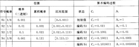
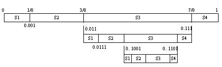
Figure 6-3 Schematic diagram of the arithmetic coding process
If the symbol sequence S3S3S2S4 is arithmetically coded, and the first symbol of the sequence is S3, we use a pointer to the third subinterval in Fig. 6-3 to represent the symbol, thereby obtaining a codeword of 0.011. Subsequent encoding will be performed within the subinterval pointed to by the previous encoding. The probability value of the [0.011, 0.111) interval is further divided into 4 parts. For the second symbol S3, the pointer points to 0.1001, and the code string becomes 0.1001. Then the subinterval corresponding to S3 is divided into 4 parts, and the third symbol is encoded.
The basic rules of arithmetic coding are as follows:
(1) Initial state: Code point (pointer pointed to) C0=0, interval width A0=1.
(2) New code point: Ci= Ci-1 + Ai-1×Pi.
Where Ci-1 is the original code point; Ai-1 is the original interval width;
The cumulative probability corresponding to the symbol coded by Pi.
New interval width Ai= Ai-1×pi
Where pi is the probability corresponding to the symbol being encoded.
According to the above rule, the process of arithmetically encoding the sequence S3S3S2S4 is as follows:
The first symbol S3:
C1=C0+A0×P1=0+1×0.011=0.011
A1=A0×p1=1×0.1=0.1
[0.011, 0.111]
The second symbol S3: C2=C1+A1×P2
=0.011+0.1×0.011=0.1001
A2=A1×p2=0.1×0.1=0.01
[0.1001, 0.1101]
The third symbol S2:
C3=C2+A2×P3=0.1001+0.01×0.001=0.10011
A3=A2×p3=0.01×0.01=0.0001
[0.10011, 0.10101]
The fourth symbol S4: C4=C3+A3×P4=0.10011+0.0001×0.111=0.1010011
A4=A3×p4=0.0001×0.001=0.0000001
[0.1010011, 0.10101)
3. Run-length coding Run Length Coding (RLC) is a very simple compression method that uses successive tokens in a data stream to represent a single token. For example, the string 5310000000000110000000012000000000000 can be compressed to 5310-10110-08120-12, where the two digits after "-" are consecutive numbers of the preceding digits of "-". The compression ratio of the run-length encoding is not high, but the encoding and decoding speed is fast, and it is still widely used, especially after the transform encoding and then the run-length encoding, which has a good effect.
6.1.5 Predictive Coding and Transform Coding 1. DPCM Principle The basic method of data compression based on statistical properties of images is predictive coding. It utilizes the spatial or temporal correlation of the image signal, predicts the current pixel with the transmitted pixels, and then encodes and transmits the difference between the predicted value and the true value, the prediction error. Currently used more linear prediction methods, known as Differential Pulse Code Modulation (DPCM), referred to as DPCM.
DPCM that utilizes intra-frame correlation (inter-pixel, inter-line correlation) is called intra prediction coding. If the luminance signal and the two color difference signals are respectively DPCM-encoded, the luminance signal is subjected to a higher sampling rate and a larger number of bits, and the color difference signal is encoded with a lower sampling rate and a smaller number of bits to form a time-division composite signal. DPCM coding is then performed, which results in a lower total code rate.
DPCM that utilizes inter-frame correlation (time correlation of adjacent frames) is called inter-prediction coding, and its coding efficiency is higher because the inter-frame correlation is greater than the intra-frame correlation. If you combine these two DPCMs, and then add variable word length coding technology, you can achieve better compression. DPCM is one of the earliest and most widely used methods in image coding technology. Its important feature is that the algorithm is simple and easy to implement in hardware. Figure 6-4(a) is a schematic diagram of the coding unit, which mainly includes a linear predictor and a quantizer.
The output of the encoder is not the sample f(m, n) of the image pixel, but the difference between the sample and the predicted value g(m, n), that is, the quantized value E of the prediction error e(m, n) (m, n). According to the analysis of the statistical characteristics of the image signal, a set of appropriate prediction coefficients is given, so that the prediction error is mainly distributed around “0â€. After non-uniform quantization, the image data is compressed by using less quantization layering. The quantization noise is not easily noticeable by the human eye, and the subjective quality of the image does not decrease significantly. Figure 6-4(b) is a DPCM decoder, the principle and the encoder are just the opposite. 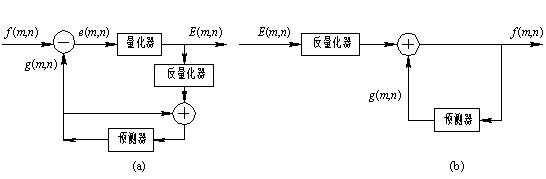
Figure 6-4 DPCM principle
(a) DPCM encoder; (b) DPCM decoder
The DPCM coding performance is mainly determined by the design of the predictor, which is to determine the order of the predictor N and the prediction coefficients. Fig. 6-5 is a schematic diagram of a fourth-order predictor, and Fig. 6-5(a) shows the positional relationship between the input pixel and the predicted pixel used by the predictor, and Fig. 6-5(b) shows the structure of the predictor.
It can be equipped with different type of storage battery such as lead acid battery, Nickel Cadmium Battery, silver zinc battery, Lithium Ion Battery and other storage batteries, providing various output voltage classes.
Built-in storage battery and charger, equipped with the function of over-charge and over-discharge protection and capacity display. It is used as working power supply for lightings, communications, laptops, and special instruments of emergency working, field working, press interviews, special vehicles and other fields.
Dc Power Supply,110V Dc Power Supply,220V Dc Power Supply,110V Dc Power Supply System
Xinxiang Taihang Jiaxin Electric Tech Co., Ltd , http://www.agvchargers.com